Python in Finance and Quantitative Analysis
In this topic, we will explore how Python is extensively used in the field of finance and quantitative analysis. From basic financial calculations to advanced algorithmic trading strategies, Python has become an indispensable tool for professionals in the finance industry. We will cover various topics, starting from the basics of financial data manipulation and analysis to advanced topics like quantitative modeling and algorithmic trading.
Introduction to Financial Data Analysis with Python
What is Financial Data?
Financial data refers to the quantitative information that reflects the financial performance and position of an entity. This data is crucial for stakeholders, including investors, management, and regulators, as it helps them assess the viability and profitability of a business.
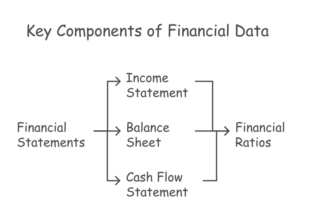
Key Components of Financial Data
Income Statement: This document summarizes the revenues, expenses, and profits over a specific period. It provides insights into a company’s operational efficiency and profitability.
Balance Sheet: A snapshot of a company’s financial position at a specific point in time, the balance sheet lists assets, liabilities, and equity. It helps stakeholders understand what the company owns and owes.
Cash Flow Statement: This statement tracks the flow of cash in and out of a business, categorizing it into operating, investing, and financing activities. It is essential for assessing liquidity and cash management.
Financial Ratios: These are metrics derived from financial statements that help analyze a company’s performance. Common ratios include the current ratio, debt-to-equity ratio, and return on equity.

Code Example: Loading Financial Data with Pandas
					import pandas as pd

# Load stock price data
stock_data = pd.read_csv('stock_prices.csv')

# Display the first few rows of the data
print(stock_data.head())
Explaination:
This code snippet demonstrates how to load financial data from a CSV file using Pandas and display the first few rows of the data.
Basic Financial Calculations
Python allows us to perform basic financial calculations such as calculating returns, volatility, and moving averages. These calculations form the foundation for more advanced analysis and modeling techniques.
Code Example: Calculating Returns
					# Calculate daily returns
stock_data['Returns'] = stock_data['Close'].pct_change()

# Display the first few rows of the returns data
print(stock_data['Returns'].head())
Explaination:
This code calculates the daily returns of a stock based on its closing prices.
Quantitative Analysis and Modeling
Quantitative analysis is a systematic approach that employs mathematical models and statistical techniques to analyze numerical data. It is widely used in finance for risk assessment, portfolio management, and pricing of financial instruments. In economics, quantitative analysis helps in understanding market trends, consumer behavior, and economic indicators.
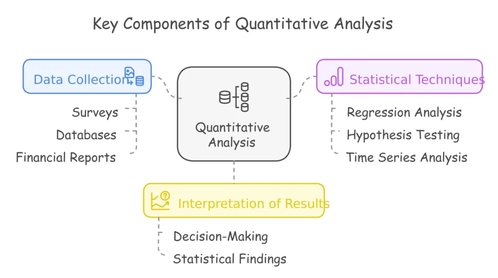
Key Components of Quantitative Analysis
Data Collection: Gathering relevant data from various sources, including surveys, databases, and financial reports.
Statistical Techniques: Utilizing methods such as regression analysis, hypothesis testing, and time series analysis to interpret data.
Interpretation of Results: Drawing conclusions based on statistical findings to inform decision-making.

Modeling Techniques
Modeling is an essential aspect of quantitative analysis, allowing analysts to simulate real-world scenarios and predict future events. Various modeling techniques are employed, including:
1. Linear Models
Linear models assume a linear relationship between variables. They are commonly used for regression analysis to predict outcomes based on independent variables.
2. Time Series Models
Time series models analyze data points collected or recorded at specific time intervals. These models are crucial for forecasting future values based on historical trends.
3. Simulation Models
Simulation models use random sampling and statistical algorithms to mimic the behavior of complex systems. They are particularly useful in risk assessment and decision-making under uncertainty.
Applications of Quantitative Analysis and Modeling
Quantitative analysis and modeling have diverse applications across various industries:
Finance: Portfolio optimization, risk management, and derivative pricing.
Healthcare: Predictive modeling for patient outcomes and resource allocation.
Marketing: Customer segmentation and sales forecasting.
Supply Chain Management: Inventory optimization and demand forecasting.
Quantitative Modeling
Quantitative modeling involves using mathematical and statistical techniques to analyze financial data and make predictions about future outcomes. Python provides libraries like SciPy and statsmodels for performing quantitative analysis.
Code Example: Linear Regression for Stock Returns
					from scipy.stats import linregress

# Perform linear regression on stock returns
slope, intercept, r_value, p_value, std_err = linregress(stock_data['Returns'], benchmark_data['Returns'])

# Display the regression results
print("Slope:", slope)
print("Intercept:", intercept)
print("R-squared:", r_value**2)
Explanation:
This code snippet demonstrates how to perform linear regression analysis on stock returns and benchmark returns using SciPy.
Algorithmic Trading Strategies
Python is widely used for developing and backtesting algorithmic trading strategies. Libraries like Backtrader and PyAlgoTrade provide tools for building and testing trading strategies using historical market data.
Code Example: Moving Average Crossover Strategy
					# Implement a simple moving average crossover strategy
def moving_average_crossover(data, short_window, long_window):
    short_ma = data['Close'].rolling(window=short_window).mean()
    long_ma = data['Close'].rolling(window=long_window).mean()
    signal = np.where(short_ma > long_ma, 1, 0)
    return signal

# Apply the strategy to stock data
signal = moving_average_crossover(stock_data, short_window=50, long_window=200)

# Display the trading signals
print(signal)
Explanation:
- This code demonstrates how to implement a simple moving average crossover strategy to generate buy and sell signals based on historical stock price data.
Risk Management and Portfolio Optimization
Risk Metrics
Risk management is crucial in finance to minimize potential losses and optimize returns. Python allows us to calculate various risk metrics such as Value at Risk (VaR) and Conditional Value at Risk (CVaR) to assess and manage risk effectively.
Code Example: Calculating VaR and CVaR
					# Calculate VaR and CVaR using historical simulation
VaR_95 = np.percentile(returns, 5)
CVaR_95 = returns[returns < VaR_95].mean()

# Display the results
print("VaR (95%):", VaR_95)
print("CVaR (95%):", CVaR_95)
Explanation:
This code snippet demonstrates how to calculate VaR and CVaR using historical simulation techniques in Python.
Portfolio Optimization
Portfolio optimization involves constructing an optimal investment portfolio that maximizes returns while minimizing risk. Python provides libraries like cvxpy for solving optimization problems and scipy.optimize for numerical optimization.
Code Example: Mean-Variance Portfolio Optimization
					import cvxpy as cp

# Define optimization variables
weights = cp.Variable(num_assets)

# Define the objective function (minimize portfolio risk)
objective = cp.Minimize(cp.quad_form(weights, cov_matrix))

# Define the constraints (sum of weights equals 1)
constraints = [cp.sum(weights) == 1]

# Solve the optimization problem
problem = cp.Problem(objective, constraints)
problem.solve()

# Display the optimal portfolio weights
print("Optimal Portfolio Weights:", weights.value)
Explanation:
This code snippet demonstrates how to perform mean-variance portfolio optimization using convex optimization techniques in Python.
Real-World Applications and Case Studies
Case Study: Predictive Modeling for Stock Prices
In this case study, we’ll build a predictive model for forecasting stock prices using machine learning techniques like linear regression and random forests.
Code Example: Predicting Stock Prices with Linear Regression
					from sklearn.linear_model import LinearRegression
from sklearn.model_selection import train_test_split

# Split data into training and testing sets
X_train, X_test, y_train, y_test = train_test_split(features, target, test_size=0.2)

# Train a linear regression model
model = LinearRegression()
model.fit(X_train, y_train)

# Make predictions
predictions = model.predict(X_test)

# Evaluate the model
mse = mean_squared_error(y_test, predictions)
print("Mean Squared Error:", mse)
Explanation:
- This code snippet demonstrates how to build and evaluate a linear regression model for predicting stock prices using scikit-learn.
Python has revolutionized the field of finance and quantitative analysis by providing powerful tools and libraries for handling financial data, performing complex calculations, and developing sophisticated trading strategies. Happy coding! ❤️
