Pie Charts in Matplotlib
]Pie charts are effective visualizations for displaying the proportional distribution of categorical data. In this topic, we will explore pie charts in Matplotlib, covering everything from basic creation to advanced customization.
Introduction to Pie Charts
What is a Pie Chart?
A pie chart is a circular statistical graphic divided into slices to illustrate numerical proportions.
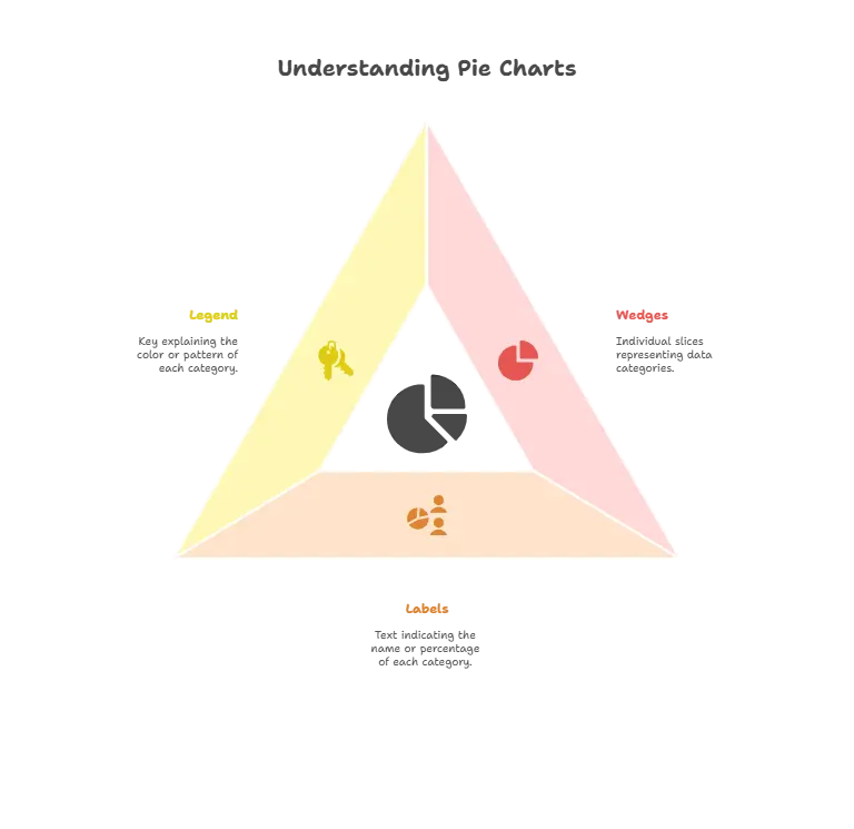
Components of a Pie Chart:
- Wedges: Individual slices representing data categories.
- Labels: Text indicating the name or percentage of each category.
- Legend: Key explaining the color or pattern of each category.

Creating a Basic Pie Chart
Example:
					import matplotlib.pyplot as plt

# Data
sizes = [20, 30, 40, 10]
labels = ['A', 'B', 'C', 'D']

# Create a basic pie chart
plt.pie(sizes, labels=labels, autopct='%1.1f%%')

# Add title
plt.title('Basic Pie Chart')

# Show the plot
plt.show()
Explanation:
- We use the
plt.pie()function to create a basic pie chart. - The
sizeslist contains the numerical values for each category, and thelabelslist contains the corresponding labels. - The
autopctparameter specifies the format of the percentage labels displayed on each wedge.
Customizing Pie Charts
Example:
					# Colors
colors = ['gold', 'yellowgreen', 'lightcoral', 'lightskyblue']

# Explode
explode = (0, 0.1, 0, 0)  # Explode the 2nd slice

# Create a customized pie chart
plt.pie(sizes, explode=explode, labels=labels, colors=colors, autopct='%1.1f%%', shadow=True)

# Add title
plt.title('Customized Pie Chart')

# Equal aspect ratio ensures that pie is drawn as a circle
plt.axis('equal')

# Show the plot
plt.show()
Explanation:
- We customize the pie chart by specifying colors, exploding a slice, adding shadows, and setting an equal aspect ratio.
- The
colorslist defines the color for each slice. - The
explodetuple determines how much each wedge is separated from the center of the pie.
Nested Pie Charts
Example:
					# Data for nested pie chart
sizes_outer = [30, 20, 50]
sizes_inner = [10, 15, 25]

# Create a nested pie chart
plt.pie(sizes_outer, labels=labels[:3], radius=1.5, colors=colors, autopct='%1.1f%%', startangle=90)
plt.pie(sizes_inner, radius=1, colors=colors[:3], autopct='%1.1f%%', startangle=90)

# Add a circle at the center to make it look like a donut chart
centre_circle = plt.Circle((0,0),0.7,fc='white')
fig = plt.gcf()
fig.gca().add_artist(centre_circle)

# Add title
plt.title('Nested Pie Chart')

# Equal aspect ratio ensures that pie is drawn as a circle
plt.axis('equal')

# Show the plot
plt.show()
Explanation:
- We create a nested pie chart by plotting two pie charts on the same axis.
- The
radiusparameter controls the size of the outer and inner pies. - Adding a white circle at the center creates the appearance of a donut chart.
Exploring Advanced Pie Chart Features
3D Pie Charts
Matplotlib also supports the creation of 3D pie charts, which add depth to the visualization.
Example:
					from mpl_toolkits.mplot3d import Axes3D

# Create a 3D pie chart
fig = plt.figure()
ax = fig.add_subplot(111, projection='3d')

ax.pie(sizes, labels=labels, autopct='%1.1f%%', startangle=90)

# Add title
plt.title('3D Pie Chart')

# Show the plot
plt.show()
Explanation:
- We import
Axes3Dfrommpl_toolkits.mplot3dto enable 3D plotting. - By specifying
projection='3d'when creating the subplot, we create a 3D plot. - The rest of the code is similar to creating a 2D pie chart.
Donut Charts with Text Annotations
We can enhance donut charts by adding text annotations to provide additional information.
Example:
					# Data for donut chart with annotations
sizes = [30, 20, 50]
labels = ['A', 'B', 'C']

# Create a donut chart with annotations
plt.pie(sizes, labels=labels, colors=colors, autopct='%1.1f%%', startangle=90)

# Draw a circle at the center
centre_circle = plt.Circle((0,0),0.7,fc='white')
fig = plt.gcf()
fig.gca().add_artist(centre_circle)

# Add annotations
plt.annotate('Category A', xy=(0, 0), xytext=(-0.6, 0.6),
             arrowprops=dict(facecolor='black', shrink=0.05))
plt.annotate('Category B', xy=(0, 0), xytext=(0.6, 0.6),
             arrowprops=dict(facecolor='black', shrink=0.05))
plt.annotate('Category C', xy=(0, 0), xytext=(0, -0.8),
             arrowprops=dict(facecolor='black', shrink=0.05))

# Add title
plt.title('Donut Chart with Annotations')

# Equal aspect ratio ensures that pie is drawn as a circle
plt.axis('equal')

# Show the plot
plt.show()
Explanation:
- We use the
annotatefunction to add text annotations with arrows pointing to each category. - The
xyparameter specifies the position of the arrow’s tip, andxytextdetermines the position of the annotation text relative to the arrow.
Pie charts are powerful tools for visualizing categorical data distributions. By understanding how to create and customize pie charts in Matplotlib, you can effectively communicate proportions and insights in your data. Experiment with different parameters and styles to create visually appealing and informative pie charts tailored to your specific needs. Happy Coding!❤️
